Flow Matching
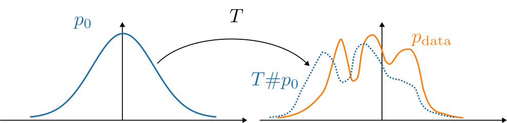
Let $p_0 = \mathcal{N}(0, I)$ and $p_1 = p_\text{data}$ be from a complex data distribution. Flow matching learns a velocity field that gradually moves samples from $p_0$ to $p_1$.
Existing flow matching tutorials either focus only on the simple $x_t = (1-t)x_0 + tx_1$ formulation without explaining why it makes mathemtical sense, or present the theory in a dense, textbook-like way. This post aims to bridge that gap. Starting from the flow-based view of generative modeling, it cohesively shows how moving probability mass from noise to data naturally leads to the flow matching objective. Readers with college-freshman-level knowledge of multivariable calculus, probability, linear algebra, and basic machine learning should be able to follow.
0. Generative Modeling
In generative modeling, we want to create new samples that look like the data we have seen. We have samples from a complex distribution $p_\text{data}$, such as images and audio, but we do not know an explicit rule for sampling new examples from it. On the other hand, we can easily sample noise from a simple distribution:
$$p_0 = \mathcal N(0, I).$$
Thus, the goal is to learn a transformation from easy-to-sample noise to realistic data samples:
$$x_0 \sim p_0 \quad \longrightarrow \quad x_1 \sim p_{\text{data}}.$$
1. Normalizing Flow
A normalizing flow is one way to parameterize this transformation. It induces a more complex distribution over $x$ from $z \sim p_0$ by applying an invertible transformation $x = f_\theta(z)$.
The probability density for $x$ is given by the change-of-variables formula for PDFs:
$$p_1(x) = p_0(f_\theta^{-1}(x))\left|\det\frac{\partial f_\theta^{-1}(x)}{\partial x}\right|.$$
Since Jacobian determinants represent a transformation's volume change, multiplying with their absolute value represents how density changes per value of $x$ after the transformation. Then, taking log and writing $x = f_\theta(z)$:
$$\log p_1(x) = \log p_0(z) - \log\left|\det\frac{\partial f_\theta(z)}{\partial z}\right|.$$
So a normalizing flow must satisfy two things:
- $f_\theta$ must be invertible;
- the Jacobian determinant must be tractable, i.e. computable by an efficient algorithm.
2. Planar Flow
A classic example of an invertible $f_\theta$ that has a tractable Jacobian determinant is a planar flow:
$$f_\theta(x) = x + uh(w^Tx+b)$$
where $x, u, w \in \mathbb{R}^d$, $b \in \mathbb{R}$. Its Jacobian is cheap by a simple chain rule:
$$\det \frac{\partial f_\theta{(x)}}{\partial x} = 1 + (h'(w^Tx + b)w)^Tu.$$
Strictly speaking, planar flows require a constraint on the parameters to guarantee invertibility; here we focus on the form because it gives a simple example of a tractable Jacobian.
However, it is not expressive, i.e. cannot represent very complex PDF transformations, as it only moves points along one direction $u$, controlled by one scalar nonlinear gate.
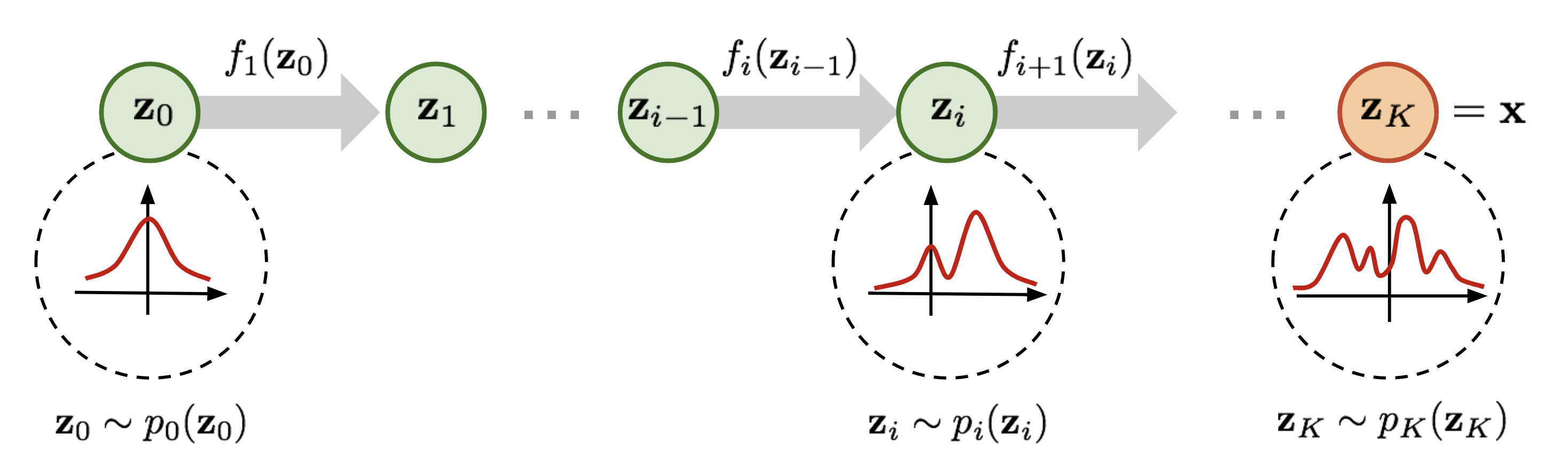
To increase expressivity, we can compose many planar flow layers:
$$x_K = f_K \circ f_{K-1} \circ \cdots \circ f_1(z).$$
By the chain rule, the density update becomes:
$$\log p_K(x_K) = \log p_0(x_0) - \sum^K_{k=1}\log\left|\det\frac{\partial f_k(x_{k-1})}{\partial x_{k-1}}\right|.$$
However, since each planar layer is a scalar projection $w^T x + b$, approximating a complicated distribution may need a lot of stacked planar layers, which is inefficient. The layer-wise nature of the stack makes it a discrete normalizing flow.
In ordinary neural networks, we can use almost arbitrary nonlinear transformations. But because normalizing flows require invertibility and tractable Jacobian determinants, their model family can be less expressive than unconstrained neural networks. This motivates continuous normalizing flows, where a more general neural network parametrizes a velocity field rather than an explicitly invertible layer.
3. Continuous Normalizing Flow
Consider a planar flow:
$$x' = f_\theta(x) = x + uh(w^Tx+b).$$
Since $u$ is a learnable parameter vector, we can reparametrize it as $u = \Delta t\tilde{u}$. Then:
$$x' = x + \Delta t\tilde{u}h(w^Tx+b).$$
Now, define a velocity field $v_t(x) = \tilde{u}_t h(w_t^T x + b_t)$, then:
$$x_{t+\Delta t} = x_t + \Delta t\ v_t(x_t).$$
This is exactly the forward Euler discretization, or Euler's method, for an ordinary differential equation (ODE):
$$\frac{dx_t}{dt} = v_t(x_t).$$
As $\Delta t \rightarrow 0$, the tiny flow layers become a continuous-time transformation. Hence, this is called a continuous normalizing flow (CNF).
The CNF defines the transformation through an initial-value-problem ODE with initial condition $x_0 = z$. Solving the ODE from $t=0$ to $t=1$ gives:
$$x_1 = \phi_1(x_0)$$
where $\phi_t$ is the flow map. The flow map satisfies:
$$\frac{d}{dt}\phi_t(x) = v_t(\phi_t(x))$$
where $\phi_0(x) = x$. Hence, we obtain $x_t = \phi_t(x)$. This mapping is invertible as we can solve the ODE backward in time, i.e. from $t=1$ back to $t=0$.
For discrete normalizing flows, the probability density evolution goes as:
$$\log p_1(x) - \log p_0(x) = - \log\left|\det\frac{\partial f_\theta(z)}{\partial z}\right|.$$
For continuous normalizing flows,
$$\frac{d}{dt} \log p_t(x_t) = -\nabla \cdot v_t(x_t).$$
This derivative is taken along a particle trajectory $x_t$, not a fixed point $x$. Intuitively, the divergence tells whether the velocity field locally expands or compresses volume. The velocity field here represents the velocity of particles carrying probability mass from $p_t$ to $p_{t+\Delta t}$. If $\nabla \cdot v_t(x_t) > 0$, then nearby particles are moving away from each other. Local volume expands, so density decreases; therefore there is a negative sign to make $\frac{d}{dt} \log p_t(x_t) < 0$ in this case.
A velocity field $v_t$ defines how individual samples move at time $t$. If we start with many samples from a simple distribution $p_0$ and move them according to the field, we can estimate the complex distribution $p_\text{data}$. The distribution of the moved samples at time $t$ is $p_t$, and a whole collection of distributions indexed by time $\{p_t\}_{t\in[0, 1]}$ gives a probability path.
There are infinitely many probability maps connecting $p_0$ and $p_1$; see visualizations of probability paths and flow maps in this ICLR 2025 blog post. However, if samples move according to a velocity field $v_t$, then the density $p_t$ must change in exactly the way induced by this motion. In other words, probability mass cannot appear or disappear; it can only flow from one region to another. The transport equation enforces this conservation of probability mass:
$$\frac{\partial p_t(x)}{\partial t} + \nabla_x \ \cdot (p_t(x)v_t(x)) = 0.$$
It means the change of density over time equals the negative net outflow of probability mass. This tells us that choosing a probability path $p_t$ implicitly determines what kind of velocity field should move samples along that path.
In a CNF, one natural way to learn this velocity field is by maximum likelihood. Given a data point $x_1$, we solve the ODE backward to obtain its corresponding noise point $x_0$, while tracking how the log-density changes:
$$\log p_1(x_1) - \log p_0(x_0) = -\int_0^1\nabla_x \cdot v_\theta(x_t, t) dt.$$
This integrates the probability density evolution formula for CNF.
In practice, optimizing $v_\theta$ is expensive because training requires ODE solving and divergence/log-density computation. Here, flow matching gives a simpler training route.
4. Flow Matching
Instead of learning $v_\theta$ by log likelihood, flow matching chooses a probability path $p_t$ from noise to data, derives its velocity field, and directly trains a neural network to match that velocity field.
A natural path is a simple linear path. Sample $x_0 \sim p_0 = \mathcal{N}(0, I)$ and $x_1 \sim p_\text{data}$, define:
$$x_t = (1-t)x_0 + tx_1.$$
Differentiate this linear interpolation:
$$\frac{dx_t}{dt} = x_1 - x_0.$$
So the target velocity is $u_t = x_1 - x_0$. Then, we can train $v_\theta(x_t, t) \approx x_1 - x_0$ with the mean squared error (MSE) loss:
$$\mathcal{L}_\text{FM} = \mathbb{E}_{x_0, x_1, t}\left[\left\|v_\theta(x_t,t)-(x_1-x_0)\right\|^2\right].$$
At inference time, starting from noise $x_0 \sim \mathcal{N}(0, I)$, flow matching solves the learned ODE $\frac{dx_t}{dt} = v_\theta(x_t, t)$ using Euler's method with $N$ steps.
Note that the actual learned neural field $v_\theta(x_t, t)$ is not memorizing each pair. Under MSE, it learns the average velocity of all pairs that could pass through the same point:
$$v_\theta^*(x,t) = \mathbb{E}\left[x_1 - x_0 \mid x_t = x\right].$$
5. Conditional Generation
The flow matching objective above is unconditional. It learns to transport noise, i.e. a random sample from $\mathcal{N}(0, I)$, into an arbitrary sample from the target distribution $p_\text{data}$. However, in many generative tasks, we do not want the model to generate an arbitrary image or an arbitrary robot action. We may want to generate an image given a text prompt, or generate a robot action given the current camera observation and language instruction.
Therefore, the velocity field should depend not only on the intermediate point $x_t$ and time $t$, but also on a condition $c$, i.e. $v_\theta(x_t, t) \rightarrow v_\theta(x_t, t, c)$. The loss will then become:
$$\mathcal{L}_\text{CFM} = \mathbb{E}_{x_0, x_1, t,c}\left[\left\|v_\theta(x_t,t, c)-(x_1-x_0)\right\|^2\right].$$
The condition $c$ tells which part of the data distribution the model should transport noise toward.
Other Resources